
High Accuracy Camera Calibration for Lens and Camera Correction
- We provide optical correction coefficients from images you provide us taken with a calibration target.
- Improve your optical system performances by powerful images analysis algorithme
- Linearize the geometric distortions in the transfer fonction of the lens
- Powerful tools for metrology calibration
Product Description
The accuracy of camera calibration is key in overall accuracy of remote measurement equipment using digital cameras. At the time of writing this article, there are probably several thousand articles covering this subject in major libraries such as IEEE, SPIE and OSA , to mention just three of them. There are available probably several thousand programs for calibration the cameras with accuracy down to 0.1 pixels, which satisfy a large number of applications.
Simply explained, any real lens has geometric distortions: a straight line on the object is projected on the image sensor as a curve. For keeping this explanation simple, we look now only at the geometric distortions. In other words, we strive to project on the image sensor as close as possible to a straight line, the image of a straight line on the object.
For calibration purposes, we find more convenient to use a calibration target with features defining very accurately a grid of equally spaced circular control points or dots in both horizontal and vertical directions. The dots size can be different across the entire target, as long as they are circular and their centers are located accurately on grid nodes. Grid nodes can be defined also by a checkerboard pattern. In image analysis, it is more accurate to compute the centroid of an ellipse than the intersection points of a checkerboard pattern. For calibration purposes, it does not make any sense of using patterns other than linear. By using modern technologies available from semiconductor industry, any shape of the real calibration pattern can be physically realized with high accuracy, using any given function expressed as high order polynomial. Line is the graph of the simplest polynomial for building and also for checking-up with the lowest errors.
The difficulty is in evaluating the departure of the projected calibration pattern on image sensor from the calibration pattern on the real object.
There are several applications when camera contribution to overall error of the measuring equipment embedding these cameras can be considered negligible if camera error goes down to 0.010 pixels or less. There are not available too many methods and subroutines for camera calibration for achieving this accuracy level. Our partner developed a calibration method and a calibration Matlab program with typical accuracy of 0.004 pixels using appropriate calibration targets as mentioned above. The idea of this method is to make corrections of the real lens for converting it to an ideal lens, with no significant errors. Once the corrected lens approaches the ideal lens, the user can use the linear camera model for any imaging application. No other corrections are further necessary for compensating the lens distortions. The calibration holds as long as using the same combination of image sensor and lens. A new calibration is required when changing either the lens, or the image sensor or both.
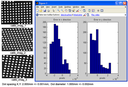
The picture above is part of an enlarged image of 150 X 150mm Dot Grid Target, Chrome/Opal, 2.000mm Spacing used for calibration, taken with 35mm lens and 1620x1220pixels camera.
It is important to mention some requirements of the images used for camera calibration:
– Gray, uncompressed, in .tif or .png format. However, only monochrome cameras are used for high accuracy measurements. Color cameras have three times less spatial resolution. Moreover, mosaicing/demosaicing algorithms associated with color cameras reduce even more their spatial resolution.
– Calibration targets must be free of dust and other particles when shooting the calibration images.
– Calibration images must have reasonable contrast.
– Notice the ellipse shape of control points (dots), coming from the regular projection. However, their centroids are held on the nodes of very accurately defined grid.
The example below shows the images of dot patterns used for camera calibration and shows also the histograms of X and Y calibration errors in object space, using those images for calibration. The histograms show the errors between the object points and the image of those object points on image sensor backward projected to the object space through the corrected lens.
The equations used for this calibration are based on several assumptions such as:
– There is only air in front of the lens and also in the back of the lens (image space).
– The camera model is orthographic.
– The camera model is decomposed in linear and nonlinear parts.
The calibration program requires:
– Three well focused images of the calibrated dots pattern either in .tif format or in .png format, as explained before, taken with best effort, looking at computer monitor.
– One image of the test pattern taken at normal incidence.
– One image of the test pattern taken at normal incidence, but left rotated with about 10 degrees (not critical).
– One image of the test pattern taken at normal incidence, but right rotated with about 10 degrees (not critical).
– Focal length of the lens, as specified by the vendor.
– Active area size of the image sensor and its number of elements on X and Y.
– Calibration target dots size and tolerances.
– Calibration target dots spacing and tolerances. It must be a square pattern of identical dots.
Based on these input parameters, our application iteratively computes the parameters and also performs error checking by dithering 1000 times the input parameters.
The outcome is camera intrinsic parameters:
– Scale factor.
– Effective focal length.
– Principal point.
– Radial distortion.
– Tangential distortion.
– Standard error in pixels.
– Standard deviation of the estimated intrinsic parameters.
– Number of iterations.
The iteration runs until is reached the imposed error. There are also generated histograms with X and Y errors as shown in the example above.
For obtaining the results shown in the example above, we used three images of fixed frequency distortion target with 1.000mm +/- 0.002mm dots diameter and 2.000mm +/- 0.001mm center dots spacing. The lens had f=35mm focal length. The black and white image sensor was Sony ICX274AL with 1620×1220 pixels and 0.0044mmX0.0044mm pixel size.
The reader must be aware that the calibration errors are expressed in pixels, not in absolute values. Of course, these differences cannot be infinitely small. We got 0.002 pixels the lowest value. Already 0.004 pixels is a very good value. Obviously, camera calibration error depends on the accuracy of the calibration target.
According to literature, when performing camera calibration with checkerboard pattern, the typical error is about 1.0 pixels.
Additional Features
- Increase your measurement accuracy
- Applicable for any system using optical lens, sensor CMOS or CCD and or laser
- Application: 2D mapping or 3D mapping, machine vision, dimension measurement
Call us at 1800-253-4107 or email sales@alliedscientificpro.com